Informed Search Algorithms

Informed Search Algorithms#

Informed search algorithms differ from blind search algorithms in the sense that the goal state is already known. Additionally, the algorithms use knowledge during the search in order to guide the search. This knowledge can take the form of distance to target, or incurred costs.

Minimum Spanning Tree#

Given a spanning tree $T$ in a graph $G$ with a weight $w$ and edges $E$, the weight $w$ of $T$ is the sum of weights of its edges. If $T$ has the minimum weight over all spanning trees of $G$, we call $T$ a minimum spanning tree.

Disjoint Sets#

Before going any further and introducing the algorithm that generates the minimum spanning $T$ given a graph $G$, we need to discuss disjoint sets, like set of vertices $V$. The main operations on disjoint sets which are interesting to us are finding the set containing a given element and forming the union of two sets, like having multiple sets of vertices of different spanning trees.

Parent Array#

Let’s consider a set $S$ which contains all $n = 12$ vertices of a graph, so $S = \{0, 1, 2, 3, 4, 5, 6, 7, 8, 9, 10, 11\}$. If we want to partition them into five sets for further processing, into $k = 5$ disjoint sets, imagine that these disjoint sets represent a single spanning tree in the graph. The vertices set would be $S = \{\{0, 1, 2\}, \{3, 4\}, \{5, 6, 7, 8\}, \{9, 10\}, \{11\}\}$. We need to be quick in maintaining these sets, so we need to refer to each set by the root of the given disjoint set (root of the tree).

Here we introduce the idea of maintaining a parent array that stores the parent of each element (node). The root won’t have a parent so its value in the parent array would be $-1$. Here is an example of the set above, think about them as trees in the graph.

from figures import *
disjoint_forest()

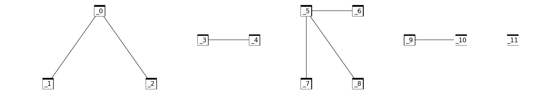
../../_images/55baf24d1030f3ad8cffb23b736e923978b21e78831a04790890dae9be862d38.png

For $V[i], i = 0,1,2, ... , 11$ $$V[i] = [0, 1, 2, 3, 4, 5, 6, 7, 8, 9, 10, 11]$$Parent[i] = [-1, 0, 0, -1, 3, -1, 5, 5, 5, 10, -1, -1]$$

So now we have a forest $F$ from the set of vertices $S$ and in $F$/$S$ we have multiple trees/disjoint sets…

Find Algorithm#

Given a vertex $i$ in a certain tree/disjoint set, we want to know the root of that tree.

FIND(Parent[0:n-1], i, r) returns The root (r) of disjoint set that contains V[i]
r ← V[i]

while Parent[r] >= 0 do

r ← Parent[r]

endwhile

return r

Minimum Spanning Tree with Kruskal’s algorithm#

KRUSKAL_MST(graph) returns a set MST contains edges of the tree
Forest ← {}
Size ← 0
for i ← 0 to n-1 do
Parent[i] ← -1
endfor
j ← 0
while Size <= n-1 and j < m do # m is the number of edges of set E = {e_i = u_iv_i | i in {1,…,m}}
j ← j + 1
FIND(Parent[0:n-1],u_j,r)
FIND(Parent[0:n-1],v_j,s)
if r ≠ s then
Forest ← Forest ∐ {e_j}
Size ← Size + 1
UNION(Parent [0:n-1],r,s)
endif endwhile MST ← Forest
return MST

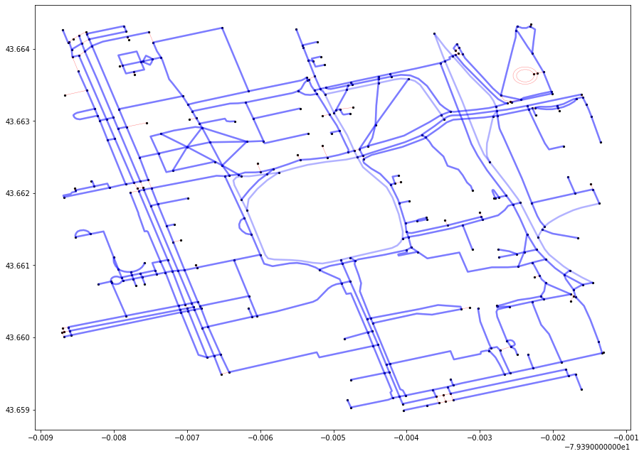
Let’s find the MST for all nodes in our search space (surrounding the University of Toronto). Here are some things to keep in mind:

The graph may seem like a one big connected component but it actually isn’t. There are one-way streets which seem to connect the adjacent nodes on the graph, but in reality they are not connected (you can go from A to B but not in reverse).
This will result in multiple MST at the end of the algorithm, one for each connected component.
There may appear to loops in the MST, which is a major violation of tree-like structures. Recall however that what may seem like loops may just be one-way streets.

import networkx
import osmnx
from matplotlib.collections import LineCollection
import matplotlib.pyplot as plt
from smart_mobility_utilities.problem import *
from utils import *
from queue import PriorityQueue

reference = (43.661667, -79.395)
G = osmnx.graph_from_point(reference, dist=300, clean_periphery=True, simplify=True)
fig, ax = osmnx.plot_graph(G)

---------------------------------------------------------------------------
ModuleNotFoundError                       Traceback (most recent call last)
Input In [2], in <cell line: 5>()
      3 from matplotlib.collections import LineCollection
      4 import matplotlib.pyplot as plt
----> 5 from smart_mobility_utilities.problem import *
      6 from utils import *
      7 from queue import PriorityQueue

ModuleNotFoundError: No module named 'smart_mobility_utilities'

# Collect x,y coordinates for each node (for visualization purposes later)
node_Xs = [float(x) for _, x in G.nodes(data='x')]
node_Ys = [float(y) for _, y in G.nodes(data='y')]

Edges = PriorityQueue()

for source, destination, data in G.edges(keys=False, data=True):
    Edges.put((data['length'],source,destination))

# Disjoint set to manage loops
nodes_set = {}
for i in Edges.queue:
    nodes_set[i[1]] = -1
    nodes_set[i[2]] = -1

# Returns -1 if the node has not been attached to another node during this run
def find_parent(node):
    r = node
    while nodes_set[r] >=0:
        r = nodes_set[r]
    return r

# The algorithm itself:
Forest = set()
Size = 0
j = 0
m = len(Edges.queue)
n = len(G.nodes)
while Size < n and j < m:
    j += 1
    # the shortest edge till this point
    edge = Edges.queue.pop()
    node1 = edge[1]
    node2 = edge[2]
    parent1 = find_parent(node1)
    parent2 = find_parent(node2)
    if parent1 != parent2:
        Forest.add(edge)
        Size += 1
        nodes_set[node1] = node2

# Visualization
sources = [edge[1] for edge in Forest]
destinations = [edge[2] for edge in Forest]

fig, ax =  plt.subplots(figsize=(15, 11))
ax.set_facecolor('w')
lines = []
colorS = []
widthS = []
for u, v, data in G.edges(keys=False, data=True):
        if 'geometry' in data:
            xs, ys = data['geometry'].xy
            lines.append(list(zip(xs, ys)))
        else:
            x1 = G.nodes[u]['x']
            y1 = G.nodes[u]['y']
            x2 = G.nodes[v]['x']
            y2 = G.nodes[v]['y']
            line = [(x1, y1), (x2, y2)]
            lines.append(line)
        if u in sources and v in destinations:
            colorS.append('b')
            widthS.append(2.5)
            continue
        if v in sources and u in destinations:
            colorS.append('b')
            widthS.append(2.5)
            continue
        colorS.append('r')
        widthS.append(0.4)    
lc = LineCollection(lines, colors=colorS, linewidths=widthS, alpha=0.3)
ax.add_collection(lc)
scat = ax.scatter(node_Xs, node_Ys,c='k', s=5)

../../_images/b4164066b7b75cc14c559be7b077169085ae25bb2af0f965dc05a290f9b7fd90.png

Hill Climbing#

The idea of the algorithm is quite simple:

Starting with a known (non-optimized) solution to a function, the algorithm checks the neighbours of that solution, and chooses the neighbour that is “more” optimized. The process is repeated until no “better” solution can be found, at which point the algorithm terminates.

While the algorithm works relatively well with convex problems, functions with multiple local maxima will often result in an answer that is not the global maximum. It also performs poorly when there are plateaus (a local set of solutions that are all similarly optimized).

HILL-CLIMBING(source,destination) return a routecurrent ← random route from source to destination
neighbours ← children of current

        while min(neighbours) < current do
        
            current ← min(neighbours)

            neighbours ← children of current
        
        return current

Here, we introduce a few new ideas.

First, we treat the route between two nodes as a function, the value of which is the distance between the two nodes. Second, we generate “children” of this function.

The function#

We need to define a function $f$ that is our target for optimization.

$f(x)$ gives us the length of a route for some given route $x \in Y$, where $Y$ is the set of all possible routes between two specific nodes.

How do we generate $x$? We could just generate random permutations between the two nodes, filtering for permutations that are feasible, and optimize $f$ over these random, sparse permutations.

However, this method is not reproducible (because the permutations change every run).

Instead, we make a deterministic policy that generates a number of $x \in Y$ by successively “failing” nodes between the source and destination nodes. We then find the shortest path between the nodes before and after the “failed” nodes.

By failing the nodes in a deterministic fashion, we can say that we have a function and neighbourhood with defined size for a certain value so we can “rigorously” conduct a local search.

To generate our initial route and children routes, we will use the smart_mobility_utilities package. You can see how these routes are generated by consulting the documentation for that package.

# Setup the Graph, origin, and destination
from smart_mobility_utilities.common import Node
from smart_mobility_utilities.viz import draw_route

reference = (43.661667, -79.395)
G = osmnx.graph_from_point(reference, dist=300, clean_periphery=True, simplify=True)

origin = Node(graph=G, osmid=55808290)
destination = Node(graph=G, osmid=389677909)

from smart_mobility_utilities.common import randomized_search, cost
from smart_mobility_utilities.children import get_children
import matplotlib.pyplot as plt
from tqdm.notebook import tqdm

# Progress bar as this algorithm can take a long time
pbar = tqdm()
# Visualize the costs over time
costs = []
# Set the number of children to generate
num_children = 20

current = randomized_search(G, origin.osmid, destination.osmid)
costs.append(cost(G,current))
print("Initial cost:",costs[0])

neighbours = get_children(G,current,num_children=num_children)
shortest = min(neighbours , key = lambda route : cost(G, route))

print("Initial min(children):",cost(G,shortest))
while cost(G, shortest) < cost(G, current):
    pbar.update(1)
    current = shortest
    neighbours = get_children(G,current,num_children=num_children)
    shortest = min(neighbours , key = lambda route : cost(G, route))
    costs.append(cost(G,current))
    print(f"Current cost:",costs[-1],"|","min(children):",cost(G, shortest))

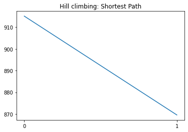
route = current

plt.xticks(range(len(costs)))
plt.title("Hill climbing: Shortest Path")
p = plt.plot(costs)
print("Final cost:",costs[-1])

Initial cost: 915.06
Initial min(children): 869.566
Current cost: 869.566 | min(children): 915.06
Final cost: 869.566

../../_images/0c7fa80b1cbdb9594f31c44609309fea6e645272eee3861d15ed7da9e0acbfdb.png

draw_route(G,route)

While the implementation above is deterministic in nature, the initial route is still randomized. That means that it’s possible to get different results across runs.

Hill climbing will generally return some decent results as there are few local optimal points in the route function. However, with larger search spaces that will naturally have more local maxima and plateaus, it will get stuck fairly quickly.

Beam Search#

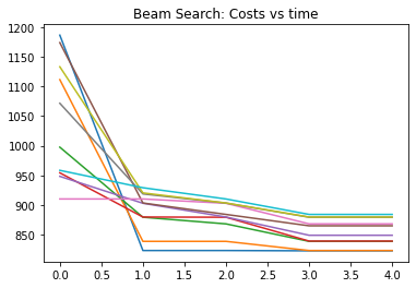
While Hill Climbing maintains a single “best” state throughout the run, beam search keeps $k$ states in memory. At each iterations, it generates the neighbours for each of the $k$ states, and puts them into a pool with the $k$ states from the original beam. It then selects the best $k$ routes from the pool to become the new beam, and this process repeats. The algorithm terminates when the new beam is equal to the old beam. As it is a local search algorithm, it is also susceptible to being stuck at local maxima.

A beam search with $k=\infty$ is the same as a BFS. Because there is the risk that a state that would lead to the optimal solution might get discarded, beam searches are considered to be incomplete (it may not terminate with the solution).

BEAM-SEARCH(source,destination,k) return a routeseen ← nil
beam ← random k routes from source to destination

        add beam to seen
pool ← children of routes in the beam with consideration of seen + beam
last_beam ← nil

        while beam is not last_beam do
        
            last_beam ← beam

            beam ← the best k routes from pool

            add beam to seen

            pool ← children of routes in the beam with consideration of seen + beam
        
return optimal route in beam

import heapq
from smart_mobility_utilities.children import get_beam
import matplotlib.pyplot as plt

# Progress bar as this algorithm can take a long time
pbar = tqdm()
# Initialize
seen = set()
k = 10
num_neighbours = 10
costs = []

beam = [randomized_search(G,origin.osmid,destination.osmid) for _ in range(k)]

# the seen routes must be converted to a tuple to be hashable to be stored in a set
for route in beam: seen.add(tuple(route))

pool = []
children = get_beam(G,beam,num_neighbours)
costs.append([cost(G,r) for r in beam])
for child in children:
    for r in child:
        if tuple(r) in seen: continue
        else: 
            pool.append(r)
            seen.add(tuple(r))
pool += beam
last_beam = None
while beam != last_beam:
    pbar.update(1)
    last_beam = beam
    beam = heapq.nsmallest(k, pool, key = lambda route: cost(G, route))
    
    for route in beam: seen.add(tuple(route))    
    
    pool = []
    children = get_beam(G,beam,num_neighbours)
    costs.append([cost(G,r) for r in beam])
    for child in children:
        for r in child:
            if tuple(r) in seen: continue
            else: pool.append(r); seen.add(tuple(r))
    pool += beam   
route = min(beam, key = lambda route : cost(G, route)) 


print("Route:",route)
print("Cost:", cost(G,route))

costs = map(list,zip(*costs))
for c in costs:
    plt.plot(c)
plt.title("Beam Search: Costs vs time")

Route: [55808290, 304891685, 55808284, 1252869817, 55808239, 389678268, 4953810915, 389678267, 24960090, 389678273, 24959523, 50885177, 389677947, 2143489692, 2480712846, 389678140, 389678139, 389678138, 3707407638, 730029011, 730029007, 2557539842, 123347786, 389678133, 389677909]
Cost: 822.524

Text(0.5, 1.0, 'Beam Search: Costs vs time')

../../_images/5fdf3ba4dfb8c9956c64129dcd143bfad9295c3a981c444cf993780909cbc508.png

draw_route(G,route)

A* Search#

A* (pronounced A-star) search is an informed search algorithm widely used in pathfinding and graph traversal.

A* works by “greedily” choosing which vertex to explore next, based on a function:

$f(V) = h(V) + g(V)$, where $h$ is a heuristic, and $g$ is the cost accrued up to that point.

A* Heuristic ← sum of straight-line distance between the node to source and node to destination
PQ ← min heap according to A* Heuristic

A*-SEARCH(source,destination) return a routefrontier ← a PQ initialized with source
explored ← empty
found ← False

        while frontier is not empty and found is False do
        node ← frontier.pop()

        add node to explored

        for child in node.expand() do
            
                if child is not in explored and child is not in frontier then
                
                if child is destination then
                    
                        route ← child.route()

                        found ← True
                    
                add child to frontier

    return route

The Heuristic#

The driving force behind A* is the selection of a new vertex (or node) to explore based on the lowest heuristic value. This heuristic value is computed by the following formula:

let $dist(x,y)$ be a function that calculates the straight line distance between two nodes $x,y$,
and let $O$ be the origin node, and $D$ be the destination node,

$h(V) = dist(V,O) + dist(V,D)$ for any given node $V$

As the sum of the distance to the origin and destination is minimized when $V$ lies on a straight line from $O$ to $D$, this heuristic prioritizes nodes which are “closer” to the straight-line distance from origin to destination.

Note

The implentation of the A* heuristic in smart_mobility_utilities defaults to calculating distances as if the Earth were flat. For local searches, this yields the best results. If the size of the search area is larger, it is better to calculate distance using the haversine_distance, which takes into account the curvature of the Earth.

This can be done by setting the distance function like so:
astar_heuristic(G,origin.osmid,destination.osmid, measuring_dist = haversine_distance)

# Get the A* Heuristic for all the nodes in the graph
from smart_mobility_utilities.problem import astar_heuristic

def A_Star(G, origin, destination):
    toOrigin, toDestination = astar_heuristic(G, origin.osmid, destination.osmid)
    route = []
    frontier = list()
    frontier.append(origin)
    explored = set()
    found = False
    while frontier and not found:   
        # choose a node based on its heuristic value
        node = min(frontier, key = lambda node : toOrigin[node.osmid] + toDestination[node.osmid])
        frontier.remove(node)
        explored.add(node)
        # expand its children
        for child in node.expand():
            if child not in explored and child not in frontier:
                if child == destination:
                    route = child.path()
                    found = True
                    continue
                frontier.append(child)
    return route

route = A_Star(G, origin, destination)
print(f"Route: {route}")
print(f"Cost: {cost(G,route)}")
draw_route(G,route)

Route: [55808290, 304891685, 55808284, 1252869817, 55808239, 389678268, 4953810915, 389678267, 24960090, 389678273, 1258698113, 389678151, 389678142, 2143489694, 389678141, 2143488528, 389678140, 389678139, 389678138, 3707407638, 6028561924, 6028561921, 389678131, 6028562356, 854322047, 389677908, 749952029, 389677909]
Cost: 839.904

Bi-Directional Search#

The purpose of bi-directional searches are to run two simultaneous, non-parallel searches; one starts at the origin and the other at the destination, with the goal of meeting somewhere in between.

This approach is more efficient because of the time complexities involved.

For example, a BFS search with a constant branching factor $b$ and depth $d$ would have an overall space complexity of $O(d^b)$. By running two BFS searches in opposite directions with only half the depth ($d/2$), the space complexity becomes instead $O((d/2)^b)+O((d/2)^b)$, which is much lower than the original $O(d^b)$.

BI-DIRECTIONAL-SEARCH(source,destination) return a route// _f for forward, _b for backward
frontier_f ← initialized with source
frontier_b ← initialized with destination
explored_f ← empty
explored_b ← empty
found ← False
collide ← False// if front overlaps with back
found ← False
altr_expand ← False// expansion direction

        while frontier_f is not empty and frontier_b is not empty and not collide and not found do
        
            if altr_expand then
            node ← frontier_f.pop()

                add node to explored_f

                for child in node.expand() do
                
                    if child in explored_f then continue

                    if child is destination then
                        
                            route ← child.route()

                            found ← True
                        
                    if child in explored_b then
                        
                            route ← child.route() + reverse(overlapped.route())

                            collide ← True
                        
                    add child to frontier_f
altr_expand ← not altr_expand

            else
            node ← frontier_b.pop()

                add node to explored_b

                for child in node.expand() do
                
                    if child in explored_b then continue

                    if child is origin then
                        
                            route ← child.route()

                            found ← True
                    
                    if child in explored_f then
                        
                            route ← reverse(child.route()) + overlapped.route()

                            collide ← True
                        
                    add child to frontier_b
altr_expand ← not altr_expand

        return route

# Using A* as search heuristic and algorithm

# define destination and origin for the backwards expansion
destination_b = origin
origin_b = destination

# get A*
toOrigin_f, toDestination_f = astar_heuristic(G, origin.osmid, destination.osmid)
toOrigin_b, toDestination_b = astar_heuristic(G, origin_b.osmid, destination_b.osmid)

route = []

f_value = lambda node: toOrigin_f[node.osmid] + toDestination_f[node.osmid]
b_value = lambda node: toOrigin_b[node.osmid] + toDestination_b[node.osmid]

frontier_f = list()
frontier_b = list()

frontier_f.append(origin)
frontier_b.append(origin_b)

explored_f = list()
explored_b = list()

collide = False
found = False
altr_expand = False # to alternate between front and back

while frontier_f and frontier_b and not collide and not found:
   
    if altr_expand:
        # remove node_f from frontier_f to expand it
        node = min(frontier_f, key = lambda node : f_value(node))
        frontier_f.remove(node)
        explored_f.append(node)
        
        for child in node.expand():
            if child in explored_f: continue
            
            if child == destination:
                route = child.path()
                found = True
                break

            # checking for collusion with the target expansion
            if child in explored_b:
                overlapped = next((node for node in explored_b if node == child))
                # we don't take the overlapped node twice
                route = child.path()[:-1] + overlapped.path()[::-1]
                collide = True
                break

            frontier_f.append(child)
        altr_expand = False
    else:
        # remove node_b from frontier_b to expand it
        node = min(frontier_b, key = lambda node : b_value(node))
        frontier_b.remove(node)
        explored_b.append(node)
        
        for child in node.expand():
            if child in explored_b: continue
            if child == destination_b:
                route = child.path()[::-1] # we reverse the list because we expand from the back
                found = True
                break

            if child in explored_f:
                overlapped = next((node for node in explored_f if node == child), None)
                route = overlapped.path()[:-1] + child.path()[::-1]
                collide = True
                break

            frontier_b.append(child)
        altr_expand = True

print("The route is \n\n",route)
route_cost = cost(G,route[:17])
second_half = route[17:]
second_half.reverse()
route_cost += cost(G,second_half)
print("Cost of the route:",route_cost)
draw_route(G,route)

The route is 

 [55808290, 304891685, 55808284, 1252869817, 55808239, 389678268, 4953810915, 389678267, 24960090, 389678273, 1258698113, 389678151, 389678142, 2143489694, 389678141, 2143488528, 389678140, 249991437, 3707407641, 24960080, 6028561924, 6028561921, 389678131, 6028562356, 854322047, 389677908, 749952029, 389677909]
Cost of the route: 827.505

Why is the cost of the final route calculated manually above? That’s because our bi-directional implementation assumes that for every edge $u,v$, there exists an edge $v,u$, but this is not the case in reality. For example, some streets may be unidirectional (i.e. one-way streets) or have turning restrictions. In our case, there is no edge that connects 2143489694 to 389678141, but an edge does exist in the reverse direction.

How can we fix this? If we assume that we are routing for the purpose of pedestrian transit, unidirectional edges essentially act as bidirectional edges and there is no real issue. We then simple need to calculate the route cost from the origin to the node before the offending node, and add the cost from the destination to the node before the offending node, as below. For more complicated routing problems involving vehicles, we can instead implement various methods to ignore unidirectional edges for the reverse path (from destination to origin) that would avoid this problem entirely.

Hierarchical Approaches#

When facing routing problems at larger scales, such as those involving entire continents or graphs with millions of nodes, it is simply implausible to use basic approaches like Dijkstra or DFS. Instead, routing algorithms “prune” the search space in order to simplify the routing problem. Additionally, routing services may choose to precompute certain routes and cache them on servers, so that response times to user queries are reasonable.

Hierarchical search algorithms prune the search space by generating admissible heuristics that abstract the search space. Read more about the general approach of hierarchical methods at Faster Optimal and Suboptimal Hierarchical Search.

In this section, we’ll give a brief overview of two hierarchical approaches that aim to solve the shortest path problem, and show how their heuristics are computed. There will also be a python implementation of the Contraction Hierarchies example.

Highway Hierarchies#

In this algorithm, the hierarchy “level” of each road/arc in the graph is calculated. This distinguishes the type of road segment (i.e. residential, national roads, highways). This is further supplemented by relevant data such as maximum designated driving speed, as well as number of turns in the road. After the heuristics are generated for the graph, the data is passed through a modified search function (bi-directional Dijkstra, A*, etc) that considers the distance to the destination and the potential expansion node class.

For example, the algorithm will generally consider highways as viable expansion nodes when it is still relatively further away from the target, and then will start to include national roads, and finally residential streets as it nears the destination.

While this approach “makes sense”, there are some disadvantages. First, the algorithm largely overlooks what kind of roads humans “prefer” to drive on. That is to say, which a highway might make sense for a given route, the user may “prefer” to take local roads (i.e. driving to a friend’s house who lives nearby). Secondly, highway hierarchies do not take into account factors such as traffic, which fluctuates often and adds significant cost to an “optimal” route.

You can learn more about contraction hierarchies here.

Contraction Hierarchies#

While the highway hierarchies algorithm may be useful for speeding up shortest path searches, it only considers three levels of road hierarchies. On the other hand, the contraction hierarchies algorithm introduced by Contraction Hierarchies: Faster and Simpler Hierarchical Routing in Road Networks has the same number of hierarchies as nodes in the graph, which is beneficial as increased number of hierarchies results in more pruning of the search space.

Contraction#

Taking any node $V$ from a graph $G$, remove $V$ as well as any connected edges.
Add any number of edges to $G$ such that the shortest distance for any pair of neighbouring nodes remains the same, even after $V$ has been removed. Below is an example:

Suppose we are contracting Node 1. By removing the node, we have now changed the shortest path for 0→2, 0→3, and 2→3. We can restore it by creating new edges. After the creation of new edges, we then reinsert any removed nodes and edges. We then update that node with its hierarchy level (which is just the order of contraction, from $1$ to $n$). See the below updated graph:

This process is then repeated for all the other nodes. In our example, no other nodes need to be contracted, as removing any one of the remaining nodes does not affect the rest of the graph in terms of shortest path. This process will form shortcuts, which allow us to search the graph much faster, as we can ignore certain nodes that have been “pruned”.

Contraction Order#

Any order for node contraction will result in a successful algorithm, however some contraction ordering systems minimizes the number of new edges added to the graph, and thus the overall running time.

To utilize this, we can employ the idea of edge difference (ED). The ED of a node is $S-E$, where $S$ is the number of new edges added if that node were to be contracted, and $E$ is the number of edges that would be deleted. Minimizing ED is equivalent to minimizing the number of new edges added to the graph, and thus improves processing time.

Example #1: Bi-directional Dijkstra with contraction#

After contracting a graph, we can run a bi-directional Dijkstra to compute all the shortest paths in the graph. Following this, any queries for the shortest path between any two nodes in the graph can be solved using a cached result.

There are some restrictions for our modified Dijkstra’s:

The forward expansion only considers arcs $u,v$, where $level(u) > level(v)$. This forms the upward graph, where only nodes with a higher contraction order can be relaxed.
The backward expansion only considers arcs $u,v$, where $level(u) < level(v)$. This forms the downward graph, where only nodes with a lower contraction order can be relaxed.

These restrictions help “prune” the search space and speed up the processing.

At the end, multiple paths are returned from source to destination, of which the shortest is selected to be the solution.

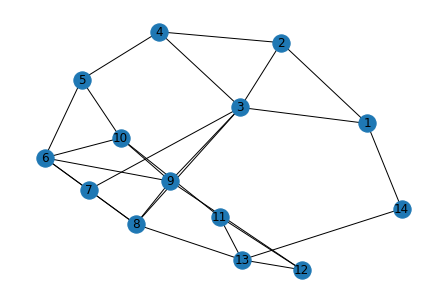
Let’s try this with the sample graph below:

import networkx
import math

G = networkx.Graph()

# Computing each contraction level requires a new graph, which is costly in terms of memory.
# To avoid this, we use a flag on every node to show its contraction state.

# Add 14 nodes
for i in range(1,15):
    G.add_node(i, contracted=False)

# Define the edges
edges = [
    (1,2,{'weight':1}),
    (1,3,{'weight':4}),
    (2,3,{'weight':5}),
    (2,4,{'weight':2}),
    (3,4,{'weight':2}),
    (3,7,{'weight':2}),
    (3,8,{'weight':1}),
    (3,9,{'weight':1}),
    (4,5,{'weight':5}),
    (5,10,{'weight':7}),
    (6,7,{'weight':4}),
    (6,8,{'weight':3}),
    (6,10,{'weight':3}),
    (6,5,{'weight':3}),
    (6,9,{'weight':1}),
    (7,8,{'weight':6}),
    (8,9,{'weight':3}),
    (8,13,{'weight':5}),
    (9,12,{'weight':1}),
    (9,10,{'weight':3}),
    (10,11,{'weight':4}),
    (11,12,{'weight':3}),
    (11,13,{'weight':4}),
    (12,13,{'weight':2}),
    (14,1,{'weight':3}),
    (14,13,{'weight':2})
]
# Add the edges to the graph and visualize it.
G.add_edges_from([*edges])
networkx.draw(G,with_labels=True)

../../_images/3cb26cadf56e15c496d2c64a9eac306fe9bfafa77f8168eaad74b235c982617e.png

Note

For this implementation we will be using two helper functions from smart_mobility_utilities.contraction.

The first is dijkstra_with_contraction, which simple runs a Dijkstra search on a graph, with the condition that the expansion nodes cannot be already contracted.

The second is calculate_edge_difference, which calculates the ED for every node in a given graph.

See the API docs for smart_mobility_utilities.contraction for more details.

We will first need to obtain the ED for the input graph:

def dijkstra_with_contraction(G, source, destination, contracted = None):
    networkx.set_node_attributes(G, {contracted: True}, 'contracted')
        
    shortest_path = dict()
    heap = list()
    
    for i in G.nodes():
        if not networkx.get_node_attributes(G, 'contracted')[i]:
            shortest_path[i] = math.inf
            heap.append(i)
    shortest_path[source] = 0
    
    while len(heap) > 0:
        
        q = min(heap, key = lambda node : shortest_path[node])
        if q == destination:
            networkx.set_node_attributes(G, {contracted: False}, 'contracted')
            return shortest_path[q]
        heap.remove(q)
        
        for v in G[q]:
            # if the node is contracted we skip it
            if not networkx.get_node_attributes(G, 'contracted')[v]:
                distance = shortest_path[q] + G[q][v]['weight']
                if distance < shortest_path[v]:
                    shortest_path[v] = distance
                    
    networkx.set_node_attributes(G, {contracted: False}, 'contracted')
    
    return math.inf # if we can't reach the destination

shortest_paths = dict()
for i in G.nodes():
    shortest_paths[i] = dict()
    for j in G.nodes():
        shortest_paths[i][j] = dijkstra_with_contraction(G, i, j)

def calculate_edge_difference(G, shortest_paths):
    edge_difference = list()
    seenBefore = list()
    
    for i in G.nodes():
        # used in edge difference calculations
        edges_incident = len(G[i])

        # we will be deleting the node entry
        # from the original shortest paths
        # dictionary so we need to save its state
        # for later iterations
        contracted_node_paths = shortest_paths[i]
        del shortest_paths[i]
        
        # excluding the node that we have just contracted
        new_graph = [*G.nodes()] 
        new_graph.remove(i)
        
        # let's compute the new shortest paths between
        # the nodes of the graph without the contracted
        # node so we can see the changes and add arcs 
        # to the graph accordingly but that is in
        # the algorithm itself 
        new_shortest_paths = dict()

        for source in new_graph:
            new_shortest_paths[source] = dict()
            for destination in new_graph:
                # path the contracted node "i" to compute new shortest paths accordingly
                new_shortest_paths[source][destination] = dijkstra_with_contraction(G, \
                                                                                    source, \
                                                                                    destination, \
                                                                                    contracted = i)
        # the add arcs to keep the graph all pairs shortest paths invariant
        shortcuts = 0

        for source in new_shortest_paths:
            # we get a copy from the original and the new shortest paths dictionary
            SP_contracted = new_shortest_paths[source]
            SP_original = shortest_paths[source]
            for destination in SP_contracted:
                # this is statement so we don't add 2 arcs
                # for the same pair of nodes 
                if [source, destination] in seenBefore: continue
                seenBefore.append(sorted((source,destination)))
                
                # if there is a difference between the original SP and
                # post-contraction SP -- just add new arc
                if SP_contracted[destination] != SP_original[destination]:
                    shortcuts += 1
        
        # let's leave the dictionary as we took it 
        # from the last iteration
        shortest_paths[i] = contracted_node_paths
        
        # this is the value of the contraction
        # heuristic for that node
        ED = shortcuts - edges_incident
        edge_difference.append((i, ED))
    return edge_difference

edge_difference = calculate_edge_difference(G,shortest_paths)
edge_difference.sort(key=lambda pair: pair[1])

edge_difference

[(8, -5),
 (10, -4),
 (5, -3),
 (7, -3),
 (11, -3),
 (14, 0),
 (2, 2),
 (1, 3),
 (6, 4),
 (13, 5),
 (4, 7),
 (12, 18),
 (3, 26),
 (9, 33)]

While this is a good start to optimizing the node contraction order, it is by no means perfect. Notice that the ED values calculated above assume the node is the only node removed from the graph. Because we are successively removing every node in the graph, the ED list will potentially become inaccurate after even the first contraction.

Recall however that any arbitrary contraction order results in a successful algorithm. While there are ED heuristics that are able to update the ED list after each contraction, each of them come with their own costs and benefits.

For the purposes of this example, our ED list will be sufficient.

# to keep track of the edges added after the algorithm finishes
edges_before = [*G.edges()]
current_graph = [*G.nodes()]

for node_ED in edge_difference:
    node = node_ED[0]
    
    # now we will contract the given node through all iterations
    networkx.set_node_attributes(G, {node: True}, 'contracted')
    
    new_graph = current_graph
    new_graph.remove(node)
    current_shortest_paths = dict()
    for source in new_graph:
            current_shortest_paths[source] = dict()
            for destination in new_graph:
                current_shortest_paths[source][destination] = dijkstra_with_contraction(G,source, destination)
                
    for source in current_shortest_paths:
        SP_contracted = current_shortest_paths[source]
        SP_original = shortest_paths[source]
        for destination in SP_contracted:
            if source == destination: continue
            if SP_contracted[destination] != SP_original[destination]:
                print("Added edge between ", source, destination," after contracting", node)
                
                G.add_edge(source, destination, weight=SP_original[destination])
                
    current_graph = new_graph

# new edges after adding additional arcs
edges_after = [*G.edges()]
print("# edges before", len(edges_before))
print("# edges after", len(edges_after))

Added edge between  1 13  after contracting 14
Added edge between  2 13  after contracting 14
Added edge between  13 1  after contracting 14
Added edge between  13 2  after contracting 14
Added edge between  1 4  after contracting 2
Added edge between  4 1  after contracting 2
# edges before 26
# edges after 29

While it may seem like edges are being added twice, this is a simple graph, so adding an edge (b,a) when there is already an edge (a,b) has no effect.

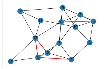
# Visualize the newly created "shortcute" on the graph

added_edges = list(set(edges_after) - set(edges_before))

# let's color these edges and draw the graph again
colors = ['r' if edge in added_edges else 'k' for edge in G.edges()]
widths = [2 if edge in added_edges else 1 for edge in G.edges()]
networkx.draw_networkx(G,with_labels=True,width=widths, edge_color=colors)

../../_images/ee4bee53d71fabaecafe7f691d08a96376addbf0e958a1e1ae6ff4d61b7050d4.png

# Reformat ED list to hierarchy for search purposes
hierarchical_order = dict()
for order, node in enumerate(edge_difference):
    hierarchical_order[node[0]] = order
    
hierarchical_order

{8: 0,
1,
2,
3,
4,
5,
6,
7,
8,
9,
10,
11,
12,
13}

Let’s now find the shortest path from $8$ to $12$, using Dijkstra’s with contraction hierarchy.

source = 8
destination = 12

# Generating the upward graph

# initializing 
SP_s = dict()
parent_s = dict()
unrelaxed_s = list()
for node in G.nodes():
    SP_s[node] = math.inf
    parent_s[node] = None
    unrelaxed_s.append(node)
SP_s[source] = 0

# dijkstra
while unrelaxed_s:
    node = min(unrelaxed_s, key = lambda node : SP_s[node])
    unrelaxed_s.remove(node)
    if SP_s[node] == math.inf: break
    for child in G[node]:
        # skip unqualified edges
        if hierarchical_order[child] < hierarchical_order[node]: continue
        distance = SP_s[node] + G[node][child]['weight']
        if distance < SP_s[child]:
            SP_s[child] = distance
            parent_s[child] = node

# Generating the downward graph

# initializing 
SP_t = dict()
parent_t = dict()
unrelaxed_t = list()
for node in G.nodes():
    SP_t[node] = math.inf
    parent_t[node] = None
    unrelaxed_t.append(node)
SP_t[destination] = 0

# dijkstra
while unrelaxed_t:
    node = min(unrelaxed_t, key = lambda node : SP_t[node])
    unrelaxed_t.remove(node)
    if SP_t[node] == math.inf: break
    for child in G[node]:
        # skip unqualified edges
        if hierarchical_order[child] < hierarchical_order[node]: continue
        distance = SP_t[node] + G[node][child]['weight']
        if distance < SP_t[child]:
            SP_t[child] = distance
            parent_t[child] = node

With these, we now merge the common settled nodes from SP_d and SP_s, and find the minimum sum of values, This is our shortest path: the collision between the forward and backward expansions.

minimum = math.inf
merge_node = None
for i in SP_s:
    if SP_t[i] == math.inf: continue
    if SP_t[i] + SP_s[i] < minimum:
        minimum = SP_t[i] + SP_s[i]
        merge_node = i

print("Minimum:",minimum)
print("Merge node:",merge_node)

Minimum: 3
Merge node: 9

# Generate the route by getting the route from source to merge node, and from destination to merge node.
def route_dijkstra(parent, node):
    route = []
    while node != None:
        route.append(node)
        node = parent[node]
    return route[::-1]
route_from_target = route_dijkstra(parent_t, merge_node)
route_from_source = route_dijkstra(parent_s, merge_node)
route = route_from_source + route_from_target[::-1][1:]
route

[8, 3, 9, 12]

Let’s compare this to networkx’s built in solver:

from networkx.algorithms.shortest_paths.weighted import single_source_dijkstra
single_source_dijkstra(G,source, destination)

(3, [8, 3, 9, 12])

Pruning#

We can actually check to see how many nodes were “pruned” from our graph, using the upward and downward graphs generated earlier.

unvisited = 0
for s_node, s_dist in SP_s.items():
    for t_node, t_dist in SP_t.items():
        if s_node == t_node and s_dist == t_dist == math.inf:
            unvisited += 1
print(f"""Skipped {unvisited} nodes from a graph with {len(G)} total nodes,
resulting in pruning {unvisited/len(G)*100}% of the nodes in our search space.""")

Skipped 7 nodes from a graph with 14 total nodes,
resulting in pruning 50.0% of the nodes in our search space.

Example #2: Equestrian Statue to Bahen Centre using Contraction Hierarchy#

We can also use the same method to calculate the shortest path between our statue and lecture hall.

Contraction hierarchies typically require incredibly powerful processing resources to run, especially when dealing with larger scales. Our ED function runs in $O(n^2)$ time, so for a graph of size 1,052 (our University of Toronto map), this requires 1,106,704 runs of dijkstra_with_contraction, which itself takes ~0.1 s per call. This would mean just calculating the ED would take 31 hours!

In order to make our example run in a more reasonable amount of time, we are going to reduce the complexity of the search space. Consider the following “simplified” road network:

import osmnx
import networkx as nx
from smart_mobility_utilities.viz import draw_route

reference = (43.661667, -79.395)

G = osmnx.graph_from_point(reference, dist=300, clean_periphery=True, simplify=True, network_type='drive_service')

fig, ax = osmnx.plot_graph(G)

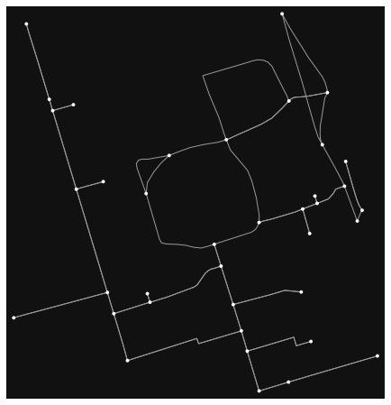
../../_images/4f9570ce47497334716fcaf8de5d7b2d6bb30463e263ba96585e29d055227212.png

This graph only contains 38 nodes and 73 edges, which is much more manageable. We can further remove any self-loops and parallel edges.

# Step 1: Remove Parallels and Loops, because Dijkstra doesn't like that
clean_G = nx.DiGraph()
clean_G.clear_edges()
for u in G.nodes:
    for v in G[u]:
        if u == v: G.remove_edge(u,v); continue
        if len(G[u][v]) > 1:
            keep = min(G[u][v], key=lambda x:G[u][v][x]['length'])
            keep = G[u][v][keep]
            clean_G.add_edge(u,v,**keep)
            continue
        clean_G.add_edge(u,v,**G[u][v][0])

print(G)
G = clean_G
print(G)

MultiDiGraph with 38 nodes and 73 edges
DiGraph with 38 nodes and 71 edges

# Using functions from smart_mobility_utilities, we can generate shortest paths and edge differences very quickly
from smart_mobility_utilities.contraction import *
sp = shortest_paths(G)
ed = edge_differences(G,sp)

edges_before = [*G.edges()]
contract_graph(G,ed,sp) # Contract the graph according to ED

edges_after = [*G.edges()]

added_edges = list(set(edges_after) - set(edges_before))
print("Added edges:", len(added_edges))

# Generate a hierarchy
hierarchical_order = dict()
for order, node in enumerate(ed):
    hierarchical_order[node] = order

Added edges: 768

# Define the start and end
start = 36603405
end = 24959560

# Generate the upward and downward graphs
up, up_SP = generate_dijkstra(G,start,hierarchical_order)
down, down_SP = generate_dijkstra(G,end,hierarchical_order,'down')

minimum = math.inf
merge_node = None

for x in up_SP:
    if x == start or x == end: continue
    if up_SP[x] == math.inf or down_SP[x] == math.inf: continue
    total = up_SP[x] + down_SP[x]
    if total < minimum: 
        minimum = total
        merge_node = x

route1 = build_route(G,start,merge_node,up)
route2 = build_route(G,end,merge_node,down)
route = route1[:-1] + route2[::-1]
print(route)
print("Cost:", round(minimum,3))

[36603405, 24960090, 24960068, 24960070, 249991437, 24960080, 5098988924, 854322047, 24959560]
Cost: 848.715

Once again, we can check to see how much the search space was pruned.

unvisited = 0
for s_node, s_dist in up_SP.items():
    for t_node, t_dist in down_SP.items():
        if s_node == t_node and s_dist == t_dist == math.inf:
            unvisited += 1
print(f"""Skipped {unvisited} nodes from a graph with {len(G)} total nodes,
resulting in pruning {round(unvisited/len(G)*100,3)}% of the nodes in our search space.""")

Skipped 2 nodes from a graph with 38 total nodes,
resulting in pruning 5.263% of the nodes in our search space.

# Reset the Graph
G = osmnx.graph_from_point(reference, dist=300, clean_periphery=True, simplify=True, network_type='drive_service')
draw_route(G,route)

While this may not look very impressive, the gains from contraction hierarchies are much more pronounced with larger graphs. Typically, larger graphs will entail more impactful contractions that significantly increases the number of pruned nodes. Contraction hierarchies allow larger graphs to run costly algorithms like Dijkstra with a negative space cost. Consider the following:

A regular Dijkstra search will need to maintain, with worst-case performance, a list of all traversed nodes and edges. This means a space complexity of $O(bd)$.
A bidirectional implementation of Dijkstra will require a space complexity of $O(bd/2) + O(bd/2)$, but has the same time complexity (unless both expansions are run simultaneously, but that has its own complications).
A contracted bidirectional Dijkstra will improve on both time and space costs, as the search space itself is modified.