
Simulated Annealing#
Let’s revisit the shortest path problem discussed previously between the Equestrian Statue and the Bahen Centre, this time using simulated annealing.
Simulated annealing is a probabilistic method of optimizing functions. Named after the process of annealing metals, simulated annealing is able to efficiently find a solution that is close to the global maximum. At its most basic level, simulated annealing chooses at each step whether to accept a neighbouring state or maintain the same state. While search algorithms like Hill Climbing and Beam Search always reject a neighbouring state with worse results, simulated annealing accepts those “worse” states probabilistically.
for num_iterations do
neighbours ← current.NEIGHBOURS
next ← randomly choose one state from neighbours
ΔE ← next.COST - current.COST
if ΔE < 0 then
route ← current
return route
Schedule#
We also need to define an annealing schedule for the algorithm. In metallurgical annealing, the key to a successful annealing is the controlled increase of temperature of a metal to a specified temperature, holding it there for some time, and then cooling it in a controlled fashion. Similarly, the probability of accepting a non-negative ΔE changes as the algorithm progresses. At first, there may be a high probability that a clearly inferior neighbour may actually be accepted, as the algorithm considers a wider search space. As the algorithm progresses however, \(T\) decreases according to a schedule until it reaches 0.
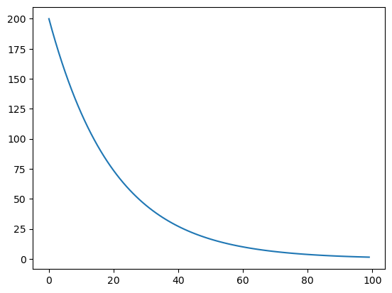
Below is an example of an annealing schedule:
import numpy as np

def exp_schedule(k=20, lam=0.005, limit=100):
    function = lambda t: (k * np.exp(-lam*t) if t <limit else 0)
    return function
import matplotlib.pyplot as plt
schedule = exp_schedule(200,0.05,10000)
T = [schedule(k) for k in range(100)]
plt.plot(T)
[<matplotlib.lines.Line2D at 0x2800fdba5c0>]
Example: Simulated annealing and the Traveling Salesman Problem#
The travelling salesman problem is one of the most famous examples of optimization.
Let’s generate a random graph of size 25. At this scale, looking for an exact solution to the TSP problem is nearly impossible (and computationally expensive).
import networkx as nx
import random
from smart_mobility_utilities.common import probability
from tqdm.notebook import tqdm

longest_edge = 0
G = nx.complete_graph(25)
for (u, v) in G.edges():
    G.edges[u, v]["weight"] = random.randint(0, 10)
    if G.edges[u, v]["weight"] > longest_edge:
        longest_edge = G.edges[u, v]["weight"]
plt.figure(figsize=(25, 25))
nx.draw(G, with_labels=True)
plt.show()
---------------------------------------------------------------------------
ModuleNotFoundError                       Traceback (most recent call last)
Input In [3], in <cell line: 3>()
      1 import networkx as nx
      2 import random
----> 3 from smart_mobility_utilities.common import probability
      4 from tqdm.notebook import tqdm
      6 longest_edge = 0

ModuleNotFoundError: No module named 'smart_mobility_utilities'
# A little utility function that finds the cost of a tour
def cost_of_tour(G, tour):
    cost = 0
    for u,v in zip(tour, tour[1:]):
        cost += G[u][v]['weight']
    cost += G[len(tour) - 1][0]['weight']
    return cost
# A function to generate neighbours and select a route
def get_neighbours(G,tour):
    # generate 5 more paths to choose from
        neighbours = list()
        for _ in range(5):
            child = tour[:]
            i = random.randint(0, len(child) - 1)
            j = random.randint(0, len(child) - 1)
            child[i], child[j] = child[j], child[i]
            neighbours.append(child)

        return random.choice(neighbours)
def simulated_annealing(
    G, initial_solution, num_iter, schedule_function, neighbour_function, cost_function, use_tqdm=False
):

    current = initial_solution
    states = [cost_function(G,initial_solution)]
    if use_tqdm: pbar = tqdm(total=num_iter)
    for t in range(num_iter):
        if use_tqdm: pbar.update()
        T = schedule_function(t)
        next_choice = neighbour_function(G,current)
        current_cost = cost_function(G, current)
        next_cost = cost_function(G, next_choice)
        delta_e = next_cost - current_cost
        if delta_e < 0 or probability(np.exp(-1 * delta_e / T)):
            current = next_choice
        states.append(cost_function(G, current))

    return current, cost_function(G,current), states
# Define the annealing schedule
num_of_iterations = 2000
schedule = exp_schedule(k=100, lam=0.005, limit=num_of_iterations)
schedules = [schedule(x) for x in range(2000)]

# Generate initial solution
initial_solution = [*G.nodes()]
random.shuffle(initial_solution)
print(f"Initial Solution: {initial_solution}")
print(f"Initial Cost: {cost_of_tour(G,initial_solution)}")
best_solution, best_cost, states = simulated_annealing(
    G, initial_solution, num_of_iterations, schedule, get_neighbours, cost_of_tour
)
print(f"Best Solution :{best_solution}")
print(f"Best Cost: {best_cost}")
plt.xlabel("# Iterations")
plt.ylabel("Cost")
plt.plot(states)
plt.show()
Initial Solution: [15, 1, 24, 8, 18, 14, 3, 9, 16, 7, 10, 6, 13, 2, 11, 21, 0, 20, 17, 22, 5, 12, 23, 4, 19]
Initial Cost: 138
Best Solution :[21, 20, 7, 4, 0, 5, 3, 1, 6, 11, 9, 12, 24, 13, 16, 8, 19, 22, 10, 18, 17, 23, 14, 15, 2]
Best Cost: 34
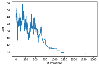
As you can see, the annealing schedule allows for more exploration at first, and then becomes more strict and generall only allows moving to a “better” solution.
Example: SA Routing Problem#
Here is an implementation of simulated annealing in python which generates a “shortest” path to solve our problem.
# Setup the Graph, origin, and destination
import osmnx
from smart_mobility_utilities.common import Node
from smart_mobility_utilities.viz import draw_route

reference = (43.661667, -79.395)
G = osmnx.graph_from_point(reference, dist=300, clean_periphery=True, simplify=True)
origin = Node(graph=G, osmid=55808290)
destination = Node(graph=G, osmid=389677909)
def get_neighbours_route(G, route):
    # Generate more paths to choose from
    neighbours = get_children(G,route,num_children=5)
    return random.choice(neighbours)
from smart_mobility_utilities.common import randomized_search, cost
from smart_mobility_utilities.children import get_children

num_iterations = 1000
schedule = exp_schedule(1000, 0.005, num_iterations)
initial_solution = randomized_search(G, origin.osmid, destination.osmid)
print (f"Initial Solution: {initial_solution}")
print(f"Initial Cost: {cost(G,initial_solution)}")
best_solution, best_cost, states = simulated_annealing(
    G,
    initial_solution,
    num_iterations,
    schedule,
    get_neighbours_route,
    cost,
    use_tqdm=True
)
Initial Solution: [55808290, 304891685, 1721866234, 9270977970, 3179025274, 4953810914, 55808233, 299625330, 389677953, 2143488335, 389677947, 2143489692, 2480712846, 389678140, 389678139, 389678138, 3707407638, 6028561924, 5098988924, 389678131, 2557539841, 389678133, 389677909]
Initial Cost: 1014.285
print(f"Best Solution: {best_solution}")
print(f"Best Cost: {best_cost}")
draw_route(G,best_solution)
Best Solution: [55808290, 304891685, 1721866234, 9270977970, 3179025274, 9270977966, 389678267, 24960090, 3108569783, 9270977968, 9270977981, 389678274, 389678273, 24959523, 50885177, 389677947, 2143489692, 2480712846, 389678140, 389678139, 389678138, 3707407638, 6028561924, 5098988924, 389678131, 2557539841, 389678133, 389677909]
Best Cost: 875.902
We can also take a look at the different states that were traversed during the annealing:
plt.xlabel("# iterations")
plt.ylabel("Cost (meters)")
plt.plot(states)
plt.show()
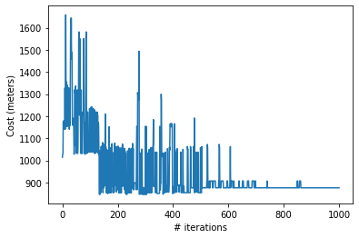
Unlike the strictly down-sloping graphs from beam search or hill-climbing, simulated annealing allows for the exploration of “worse” results, which broadens the search space.