From Road Network to Graph

From Road Network to Graph#

This section contains a non-exhaustive list of operations on geospatial data that you should familiarize yourself with. More information can be found by consulting the Tools and Python Libraries page or the respective libary’s API documentation.

Creating a Graph from a named place#

Mathematically speaking, a graph can be represented by \(G\), where

\(G=(V,E)\)

For a graph \(G\), vertices are represented by \(V\), and edges by \(E\).

Each edge is a tuple \((v,w)\), where

\(w\), \(v \in V\)

Weight can be added as a third component to the edge tuple.

In other words, graphs consist of 3 sets:

vertices/nodes
edges
a set representing relations between vertices and edges

The nodes represent intersections, and the edges represent the roads themselves. A route is a sequence of edges connecting the origin node to the destination node.

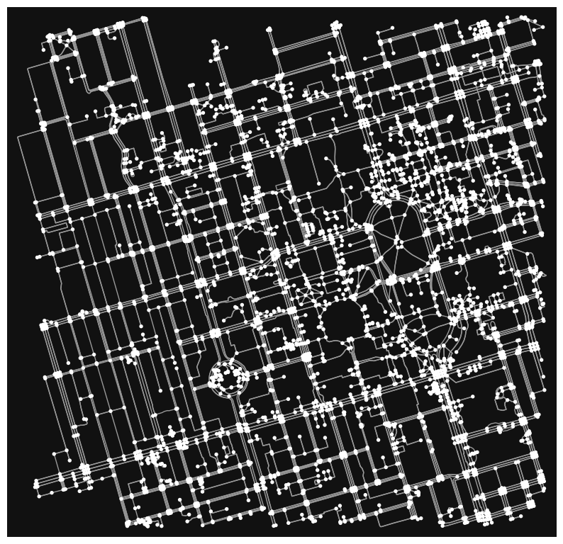
osmnx can convert a text descriptor of a place into a networkx graph. Let’s use the University of Toronto as an example:

import osmnx

place_name = "University of Toronto"


# networkx graph of the named place
graph = osmnx.graph_from_address(place_name)

# Plot the graphs
osmnx.plot_graph(graph,figsize=(10,10))

../../_images/7b96ffb1e0c98033b8213dbf7e8b728ddc691ea8942b5a0a8bc4028fe39f9f49.png

(<Figure size 1000x1000 with 1 Axes>, <AxesSubplot:>)

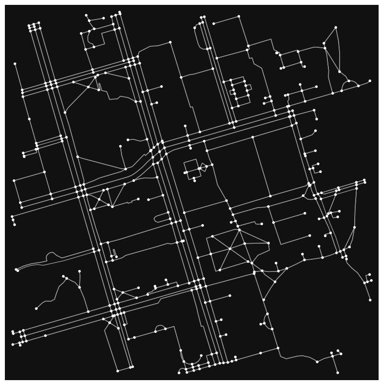
The graph shows edges and nodes of the road network surrouding the University of Toronto’s St. George (downtown Toronto) campus. While it may look visually interesting, it extends a bit too far off campus, and lacks the context of the street names and other geographic features. Let’s restrict the scope of the network to 500 meters around the university, and use a folium map as a baselayer. We will discuss more about folium later in this section.

graph = osmnx.graph_from_address(place_name, dist=300)
osmnx.folium.plot_graph_folium(graph)

Make this Notebook Trusted to load map: File -> Trust Notebook

Suppose you want to get from one location to another on this campus.

Starting at the King Edward VII Equestrian Statue near Queen’s Park, you need to cut across the campus to attend a lecture at the Bahen Centre for Information Technology. Later in this section, you will see how you can calculate the shortest path between these two points.

For now, let’s plot these two locations on the map using ipyleaflet:

from ipyleaflet import *

# UofT main building
center=(43.662643, -79.395689) 
# King Edward VII Equestrian Statue
source_point = (43.664527, -79.392442)  
# Bahen Centre for Information Technology at UofT
destination_point = (43.659659, -79.397669) 

m = Map(center=center, zoom=15)
m.add_layer(Marker(location=source_point, icon=AwesomeIcon(name='camera', marker_color='red')))
m.add_layer(Marker(location=center, icon=AwesomeIcon(name='graduation-cap')))
m.add_layer(Marker(location=destination_point, icon=AwesomeIcon(name='university',marker_color='green')))
m

Notice that the way we create maps in ipyleaflet is different from folium. For the latter, the code is as follows:

import folium
m = folium.Map(location=center, zoom_start=15)
folium.Marker(location=source_point,icon=folium.Icon(color='red',icon='camera', prefix='fa')).add_to(m)
folium.Marker(location=center,icon=folium.Icon(color='blue',icon='graduation-cap', prefix='fa')).add_to(m)
folium.Marker(location=destination_point,icon=folium.Icon(color='green',icon='university', prefix='fa')).add_to(m)
m

Make this Notebook Trusted to load map: File -> Trust Notebook

Extracting Graph Information#

Various properties of the graph can be examined, such as the graph type, edge (road) types, CRS projection, etc.

Graph Type#

type(graph)

networkx.classes.multidigraph.MultiDiGraph

Note

You can read more about MultiDiGraph here.

Edges and Nodes#

We can extract the nodes and edges of the graph as separate structures.

nodes, edges = osmnx.graph_to_gdfs(graph)

nodes.head(5)

	y	x	highway	street_count	geometry
osmid
21631731	43.664076	-79.398440	traffic_signals	4	POINT (-79.39844 43.66408)
24959527	43.664436	-79.396904	NaN	3	POINT (-79.39690 43.66444)
24959528	43.664687	-79.395701	NaN	3	POINT (-79.39570 43.66469)
24959535	43.663497	-79.400045	traffic_signals	4	POINT (-79.40004 43.66350)
24959542	43.665940	-79.401019	stop	3	POINT (-79.40102 43.66594)

edges.head(5)

			osmid	lanes	name	highway	maxspeed	oneway	reversed	length	geometry	access	service	width	tunnel
u	v	key
21631731	389678033	0	277878927	3	St George Street	tertiary	30	False	True	12.829	LINESTRING (-79.39844 43.66408, -79.39840 43.6...	NaN	NaN	NaN	NaN
	389678008	0	327452916	3	St George Street	tertiary	30	False	True	12.667	LINESTRING (-79.39844 43.66408, -79.39848 43.6...	NaN	NaN	NaN	NaN
	389677903	0	10334990	3	Hoskin Avenue	tertiary	NaN	False	True	10.351	LINESTRING (-79.39844 43.66408, -79.39839 43.6...	NaN	NaN	NaN	NaN
	389677893	0	126742589	3	Harbord Street	tertiary	40	False	True	14.564	LINESTRING (-79.39844 43.66408, -79.39847 43.6...	NaN	NaN	NaN	NaN
24959527	389678004	0	77720372	2	Devonshire Place	residential	30	False	False	8.867	LINESTRING (-79.39690 43.66444, -79.39694 43.6...	NaN	NaN	NaN	NaN

We can further drill down to examine each individual node or edge.

# Rendering the 2nd node
list(graph.nodes(data=True))[1]

(24959527, {'y': 43.6644357, 'x': -79.3969038, 'street_count': 3})

# Rendering the 1st edge
list(graph.edges(data=True))[0]

(21631731,
 389678033,
 {'osmid': 277878927,
  'lanes': '3',
  'name': 'St George Street',
  'highway': 'tertiary',
  'maxspeed': '30',
  'oneway': False,
  'reversed': True,
  'length': 12.829})

Street Types#

Street types can also be retrieved for the graph:

print(edges['highway'].value_counts())

footway                       898
service                        90
residential                    58
tertiary                       54
[footway, steps]               21
unclassified                   15
living_street                  14
pedestrian                     10
[footway, service]              4
steps                           4
[steps, footway]                3
secondary                       2
[footway, steps, corridor]      2
[footway, service, steps]       1
[steps, service, footway]       1
Name: highway, dtype: int64

GeoDataFrame to MultiDiGraph#

GeoDataFrames can be easily converted back to MultiDiGraphs by using osmnx.graph_from_gdfs.

new_graph = osmnx.graph_from_gdfs(nodes,edges)
osmnx.plot_graph(new_graph,figsize=(10,10))

../../_images/4727505727d8773a8f0df14b62a77cbc7048149d4e46a1d34a923a210db16313.png

(<Figure size 1000x1000 with 1 Axes>, <AxesSubplot:>)

Calculating Network Statistics#

We can see some basic statistics of our graph using osmnx.basic_stats.

osmnx.basic_stats(graph)

{'n': 421,
 'm': 1177,
 'k_avg': 5.59144893111639,
 'edge_length_total': 32953.49499999998,
 'edge_length_avg': 27.997871707731505,
 'streets_per_node_avg': 3.02375296912114,
 'streets_per_node_counts': {0: 0, 1: 62, 2: 1, 3: 228, 4: 126, 5: 3, 6: 1},
 'streets_per_node_proportions': {0: 0.0,
  1: 0.14726840855106887,
  2: 0.0023752969121140144,
  3: 0.5415676959619953,
  4: 0.2992874109263658,
  5: 0.007125890736342043,
  6: 0.0023752969121140144},
 'intersection_count': 359,
 'street_length_total': 16663.342,
 'street_segment_count': 594,
 'street_length_avg': 28.05276430976431,
 'circuity_avg': 1.0287183227563486,
 'self_loop_proportion': 0.0}

We can also see the circuity average. Circuity average is the sum of edge lengths divided by the sum of straight line distances. It produces a metric > 1 that indicates how “direct” the network is (i.e. how much more distance is required when travelling via the graph as opposed to walking in a straight line).

# osmnx expects an undirected graph
undir = graph.to_undirected()
osmnx.stats.circuity_avg(undir)

1.0287183227563486

Extended and Density Stats#

Density-based statistics requires knowing the area of the graph. To do this, the convex hull of the graph is required.

convex_hull = edges.unary_union.convex_hull
convex_hull

../../_images/5f9ae050669e6d19556d71fe5bf05a7c62afaa1eea7517ecb56aa27f73ede649.svg

import pandas
area = convex_hull.area
stats = osmnx.basic_stats(graph, area=area)
extended_stats = osmnx.extended_stats(graph,ecc=True,cc=True)
stats.update(extended_stats)

# Show the data in a pandas Series for better formatting
pandas.Series(stats)

---------------------------------------------------------------------------
AttributeError                            Traceback (most recent call last)
Input In [15], in <cell line: 4>()
      2 area = convex_hull.area
      3 stats = osmnx.basic_stats(graph, area=area)
----> 4 extended_stats = osmnx.extended_stats(graph,ecc=True,cc=True)
      5 stats.update(extended_stats)
      7 # Show the data in a pandas Series for better formatting

AttributeError: module 'osmnx' has no attribute 'extended_stats'

Warning

extended_stats has already been deprecated from osmnx. In the absence of an alternative, you can access these metrics directly through networkx.

CRS Projection#

You can also look at the projection of the graph. To find out more about projections, check out this section. Additionally, you can also reproject the graph to a different CRS.

edges.crs

<Geographic 2D CRS: EPSG:4326>
Name: WGS 84
Axis Info [ellipsoidal]:
- Lat[north]: Geodetic latitude (degree)
- Lon[east]: Geodetic longitude (degree)
Area of Use:
- name: World.
- bounds: (-180.0, -90.0, 180.0, 90.0)
Datum: World Geodetic System 1984 ensemble
- Ellipsoid: WGS 84
- Prime Meridian: Greenwich

merc_edges = edges.to_crs(epsg=3857)
merc_edges.crs

<Projected CRS: EPSG:3857>
Name: WGS 84 / Pseudo-Mercator
Axis Info [cartesian]:
- X[east]: Easting (metre)
- Y[north]: Northing (metre)
Area of Use:
- name: World between 85.06°S and 85.06°N.
- bounds: (-180.0, -85.06, 180.0, 85.06)
Coordinate Operation:
- name: Popular Visualisation Pseudo-Mercator
- method: Popular Visualisation Pseudo Mercator
Datum: World Geodetic System 1984 ensemble
- Ellipsoid: WGS 84
- Prime Meridian: Greenwich

Shortest Path Analysis#

Let’s revisit our trip across campus from the statue in Queen’s Park to our lecture hall at the Bahen centre.

To calculate the shortest path, we first need to find the closest nodes on the network to our starting and ending locations.

import geopandas

X = [source_point[1], destination_point[1]]
Y = [source_point[0], destination_point[0]]
closest_nodes = osmnx.distance.nearest_nodes(graph,X,Y)

# Get the rows from the Node GeoDataFrame
closest_rows = nodes.loc[closest_nodes]

# Put the two nodes into a GeoDataFrame
od_nodes = geopandas.GeoDataFrame(closest_rows, geometry='geometry', crs=nodes.crs)
od_nodes

	y	x	highway	street_count	geometry
osmid
390545921	43.665132	-79.394109	NaN	3	POINT (-79.39411 43.66513)
239055725	43.660783	-79.397878	NaN	3	POINT (-79.39788 43.66078)

Let’s find and plot the shortest route now!

import networkx

shortest_route = networkx.shortest_path(G=graph,source=closest_nodes[0],target=closest_nodes[1], weight='length')
print(shortest_route)

[390545921, 60654129, 60654119, 389678001, 389678002, 2143434369, 390550470, 127289393, 8277128565, 8277128566, 4920594801, 3996671922, 80927418, 7967019552, 127275360, 80927426, 2143468197, 2143468182, 55808564, 55808527, 130170945, 389677905, 389678182, 389677906, 50885141, 389678180, 1258706668, 2143436407, 1258706673, 2143402269, 2143402268, 1258706670, 239055725]

osmnx.plot_graph_route(graph,shortest_route,figsize=(15,15))

../../_images/40302f72082b29f7427cbdbc075a3cb57bd3a848b1fffbf9cd907c6e031af593.svg

(<Figure size 1080x1080 with 1 Axes>, <AxesSubplot:>)

Now let’s try visualizing this on a leaflet map. We’ll use the ipyleaflet library for this. Graphs rendered in ipyleaflet tend to be very slow when there are many nodes. For this reason, the code will fall back to folium if there are more than 1,500 nodes in the graph (this particular graph should have ~1,090 nodes).

Let’s make a map that shows the above route, with both starting and ending nodes shows as markers.

import ipyleaflet
import networkx

def draw_route(G, route, zoom=15):
    if len(G)>=1500:
        # Too many nodes to use ipyleaflet
        return osmnx.plot_route_folium(G=G,route=route)
    
    # Calculate the center node of the graph
    # This used to be accessible from extended_stats, but now we have to do it manually with a undirected graph in networkx
    undir = G.to_undirected()
    length_func = networkx.single_source_dijkstra_path_length
    sp = {source: dict(length_func(undir, source, weight="length")) for source in G.nodes}
    eccentricity = networkx.eccentricity(undir,sp=sp)
    center = networkx.center(undir,e=eccentricity)[0]

    # Create the leaflet map and center it around the center of our graph
    G_gdfs = osmnx.graph_to_gdfs(G)
    nodes_frame = G_gdfs[0]
    ways_frame = G_gdfs[1]
    center_node = nodes_frame.loc[center]
    location = [center_node.y,center_node.x]
    m = ipyleaflet.Map(center=location, zoom=zoom)

    # Get our starting and ending nodes
    start_node = nodes_frame.loc[route[0]]
    end_node = nodes_frame.loc[route[-1]]
    start_xy = [start_node.y, start_node.x]
    end_xy = [end_node.y,end_node.x]

    # Add both nodes as markers
    m.add_layer(ipyleaflet.Marker(location=start_xy, draggable=False))
    m.add_layer(ipyleaflet.Marker(location=end_xy, draggable=False))

    # Add edges of route
    for u,v in zip(route[0:],route[1:]):
        try:
            x,y = (ways_frame.query(f'u == {u} and v == {v}').to_dict('list')['geometry'])[0].coords.xy
        except:
            x,y = (ways_frame.query(f'u == {v} and v == {u}').to_dict('list')['geometry'])[0].coords.xy

        points = map(list, [*zip([*y],[*x])])
        ant_path = ipyleaflet.AntPath(
            locations = [*points], 
            dash_array=[1, 10],
            delay=1000,
            color='#7590ba',
            pulse_color='#3f6fba'
        )
        m.add_layer(ant_path)

    return m
draw_route(graph, shortest_route)

Retrieve buildings from named place#

Just like our graph above, we can also retrieve all the building footprints of a named place.

# Retrieve the building footprint, project it to match our previous graph, and plot it.
buildings = osmnx.geometries.geometries_from_address(place_name, tags={'building':True}, dist=300)
buildings = buildings.to_crs(edges.crs)
osmnx.plot_footprints(buildings)

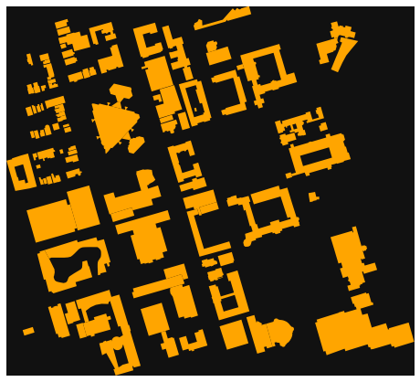
../../_images/d2fee90d06342b03887bb62440e9ba2a61f867d43925cdfbd3f6544bb79ee0ea.png

(<Figure size 576x576 with 1 Axes>, <AxesSubplot:>)

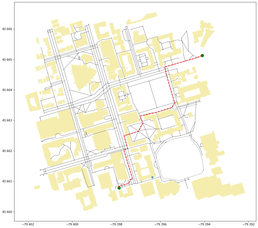
Now that we have the building footprints for the campus, let’s plot that shortest route again.

First, get the nodes from the shortest route, create a geometry from it, and then visualize building footprints, street network, and shortest route all on one plot.

from shapely.geometry import LineString

# Nodes of our shortest path
route_nodes = nodes.loc[shortest_route]

# Convert the nodes into a line geometry
route_line = LineString(list(route_nodes.geometry.values))

# Create a GeoDataFrame from the line
route_geom = geopandas.GeoDataFrame([[route_line]], geometry='geometry', crs=edges.crs, columns=['geometry'])

# Plot edges and nodes
ax = edges.plot(linewidth=0.75, color='gray', figsize=(15,15))
ax = nodes.plot(ax=ax, markersize=2, color='gray')

# Add building footprints
ax = buildings.plot(ax=ax, facecolor='khaki', alpha=0.7)

# Add the shortest route
ax = route_geom.plot(ax=ax, linewidth=2, linestyle='--', color='red')

# Highlight the starting and ending nodes
ax = od_nodes.plot(ax=ax, markersize=100, color='green')

../../_images/758087d3ec8655323824e8d5c7c30c0c53a5744677b2788cfd8cf1bf14875ca6.png