Spatial Data and Geographic Information System (GIS)#
Spatial data is any type of data that directly or indirectly references tp specific geographic locations. Examples of this data include, but are not limited to,
Locations of people, businesses, assets, natural resources, new developments, services and other built infrastructure.
Spatially distributed variables such as traffic, health statistics, demographics and weather .
Data related to environmental change –ecology, sea level rise, pollution, temperature, etc.
Data related to coordination of responses to emergencies, natural and man-made disasters – floods, epidemics, terrorism
A Geographic Information System (GIS) is a computer-based system to aid in the collection, maintenance, storage, analysis, output, and distribution of spatial data and information [2]. GIS mainly deals with two categories of data: (i.e. absolute and relative location of features) and what (i.e. the properties and attributes of those features). However, the use of GIS can be extended to include other questions such as why (i.e, why features are located where they are) and how (i.e, how these features are different from one another, and how they interact with each other).
Read Geospatial Data Files#
Geospatial data files come in a variety of formats. Below are some of the most popular file types:
Shapefiles (
.shp)GeoJSON (
.geojson)Geography Markup Language (
.gml)Google’s Keyhole Markup Language (
.kml)OpenStreetMap XML (
.osm)Comma-separated values (
.csv)
These file formats store geospatial data in different ways, and each offers various advantages and disadvantages.
For example, .shp is a widely-used file format, supported by nearly every open source and commercial GIS software, while .geojson files are natively compatible with JavaScript, making it excellent for web-based mapping applications.
Note
The above file formats are all used to represent vector data (points, edges, polygons). Raster files (i.e. photogrammetry), are typically stored as .tiff,.jp2, or .bmp files.)
Below is a typical example of opening a .shp using geopandas. This particular file was downloaded from the Province of Ontario’s Data Catalogue[3].
import geopandas as gpd

# file downloaded from https://data.ontario.ca/dataset/ontario-s-health-region-geographic-data
ontario = gpd.read_file(r"../../data/ontario_health_regions/Ontario_Health_Regions.shp")

ontario
| Shape_Leng | Shape_Area | REGION | REGION_ID | geometry | |
|---|---|---|---|---|---|
| 0 | 4.845977e+06 | 1.089122e+11 | East | 04 | MULTIPOLYGON (((-8631925.914 5449844.839, -863... |
| 1 | 3.211510e+07 | 2.232211e+12 | North | 05 | MULTIPOLYGON (((-8943097.220 5627248.576, -894... |
| 2 | 4.860262e+06 | 7.543033e+10 | West | 01 | MULTIPOLYGON (((-9204865.114 5113839.368, -920... |
| 3 | 2.755817e+06 | 3.189867e+10 | Central | 02 | MULTIPOLYGON (((-8872905.739 5371938.215, -887... |
| 4 | 2.196396e+05 | 3.715020e+08 | Toronto | 03 | MULTIPOLYGON (((-8839514.979 5425932.689, -883... |
As you can see, the Shapefile we opened contains five entries (index 0 to 4).
Geopandas typically represents data in the following format [4]:

As you can see from our table output above, this particular shapefile contains Shape_Leng, Shape_Area, REGION, and REGION_ID as data columns, and stores the features as MULTIPOLYGON.
Note
The regions in this file are stored as multipolygon because some regions contain multiple land masses. You can read more about shapely multipolygons here.
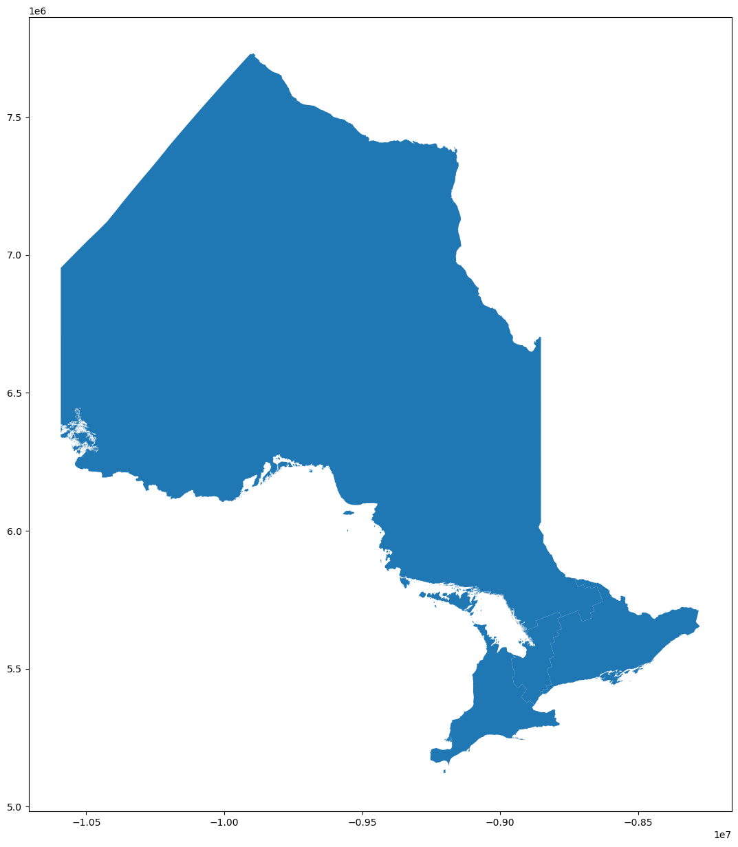
Now that we have the file loaded into geopandas, we can plot it to visualize and analyze the data.
ontario.plot(figsize=(15,15))
<AxesSubplot:>
We can also inspect metadata about the dataset. This includes column names, data types, as well as size (in memory) of the dataframe.
ontario.info()
<class 'geopandas.geodataframe.GeoDataFrame'>
RangeIndex: 5 entries, 0 to 4
Data columns (total 5 columns):
 #   Column      Non-Null Count  Dtype
---  ------      --------------  -----
 0   Shape_Leng  5 non-null      float64
 1   Shape_Area  5 non-null      float64
 2   REGION      5 non-null      object
 3   REGION_ID   5 non-null      object
 4   geometry    5 non-null      geometry
dtypes: float64(2), geometry(1), object(2)
memory usage: 328.0+ bytes